Time series ML | Wake-word detection with DSCNNs

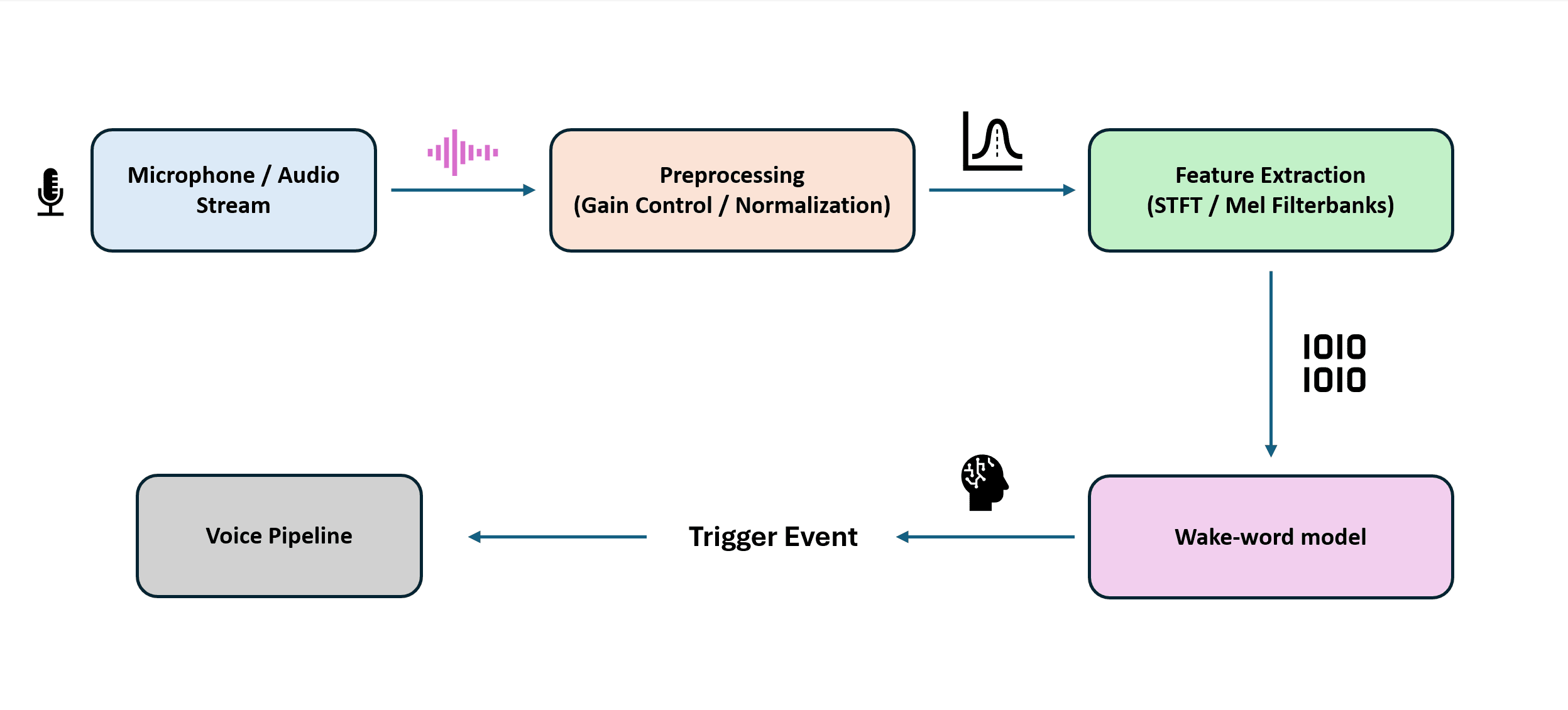
Wake-word detection or key word spotting (KWS) is an excellent time series problem in Machine learning. To be functional, it must be fast, accurate, and robust in noisy environments. In most setups, this detection is done with lightweight models running directly on the device. However, Alexa is known for having a 2 stage approach where the on-device detector triggers and then a short snippet of audio is sent to the cloud for verification on a more powerful model. To avoid sending our voice data to the cloud we must find a reliable solution.

What the model does

Classifies short audio windows (approx 1s) as either containing the wake-word or not. This will then trigger the rest of the voice pipeline (STT -> LLM -> TTS)

Why it matters

This is the only part of Ella that is always on and listening. It is crucial to be both accurate and efficient so that it can run locally without draining unnecessary power

Custom Dataset

I build a wake-word dataset from real microphone recordings in various envirnoments including near field, far field and with background noise. These samples were segmented into 1 second windows and labeled as positive or negative. I also used augmentation techniques like noise mixing and timeshifting for robustness.

Why DSCNN instead of CNN?

Standard convolutional neural networks (CNNs) work well for keyword spotting but they are often heavier than necessary for edge devices. Depthwise seperable convolutional neural networks (DSCNNs) replace expensive convolutions with a two step factorization (depthwise + pointwise), dramatically reducing compute while keeping accuracy similar in many situations.

Source (images)

Standard CNN convolution
A standard convolutional layer jointly learns spatial filtering and cross channel mixing in one go. This is powerful but expensive especially for always on audio processing running on a CM5.

Depthwise separable convolution (DSCNN)
Depthwise convolutions handle spatial filtering per channel and then are followed by a 1×1 pointwise convolution to mix channels. These often reduce parameters by up to 80% which in turn reduces latency while still maintaining a comparable accuracy.

Why it’s cheaper

Let us define the following:
Input: H_in x W_in x C_in
Kernel: K_h x K_w
Output channels: C_out
Output map: H_out x W_out

Standard convolution learns spatial filtering and channel mixing in one step. The multiply-accumulate operations (MACs) scales as:
MACs_conv = H_out x W_out x C_out x (K² x C_in)
(and parameters scale as K² x C_in x C_out)

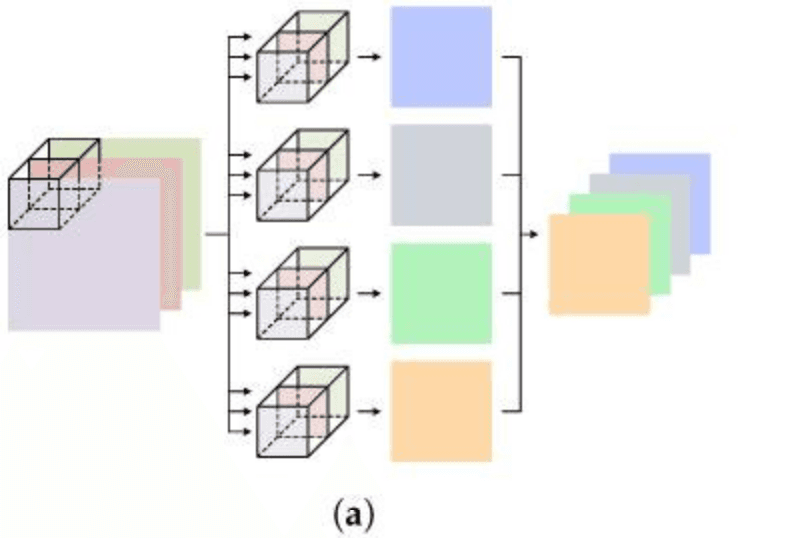
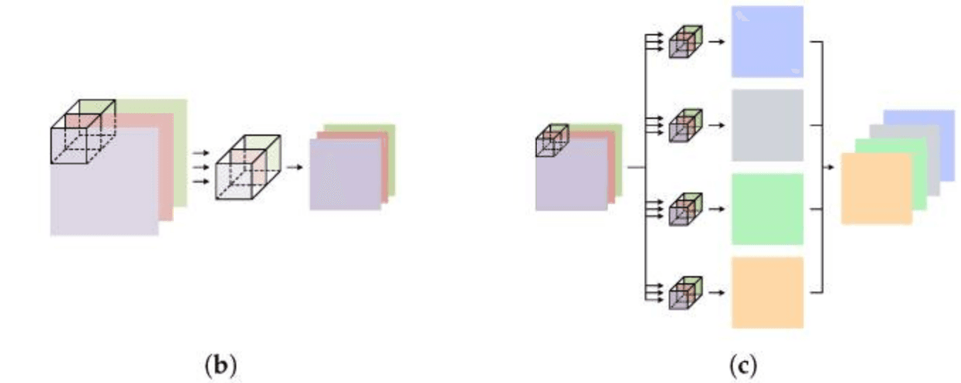
Depthwise-separable convolution splits this into:
1) Depthwise (one K x K filter per input channel): MACs_dw = H_out x W_out x C_in x K²
2) Pointwise (1x1 channel mixing): MACs_pw = H_out x W_out x C_in x C_out

Total:
MACs_DS = H_out x W_out x (C_in x K² + C_in x C_out)

Compared to standard conv, the DS-CNN cost ratio is approximately:
MACs_DS / MACs_conv ≈ 1/C_out + 1/K²
So with K = 3 (K² = 9) and depending on channel widths, DSCNNs are around 7-9x cheaper

Full derivation

Speech features (log-mel) and how the model “sees” audio

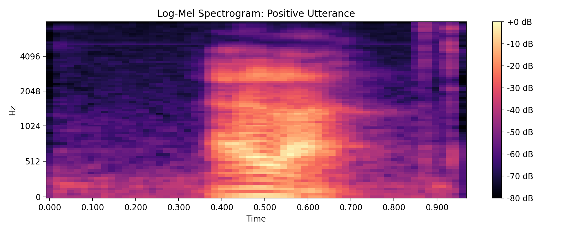
Raw waveforms are information dense but expensive to learn from, and are generally considered overkill for ML purposes. Instead we can compress this information into what is called a log-mel spectrogram which is a time-frequency representation with usually around 30-60 frequency bins. The frequencies are grouped using a mel scale which perceptually aligns with human hearing.

Feature pipeline

1) Window audio: We collect short 10-20ms frames of audio with an overlap
2) Short Time Fourier Transform (STFT): We convert each window into frequency bins each associated with a complex coefficient that represents the magnitude and phase of that frequency component in the window
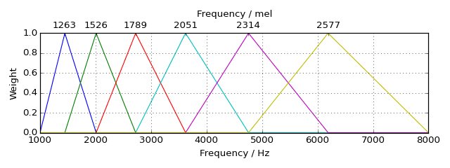
3) Mel filterbank: We apply a set of overlapping triangular filters that are narrower at lower frequencies and wider at higher frequencies. We do this because human hearing is more sensitive to lower frequencies so granularity is more important there.
4) Log compression: We shrink the large dynamic range of the mel spectrogram by applying a logarithm. This prevents large magnitude frequency bins from overwhelming quiter (likely more important) details. This allows for easier learning and also better aligns with actual human perception of loudness which is logarithmic in nature

Example log-mel spectrogram for a wake word — Mel Filterbanks

Time series ML | Wake-word detection with DSCNNs

Why DSCNN instead of CNN?

Speech features (log-mel) and how the model “sees” audio

Feature pipeline

Demo